How to import data from an Access database?


If you have an Access database that you want to manipulate using Excel, then you can import it. To do this follow the steps below. 


1. Go to the Data tab and select Get Data. 


2. Select From Database


3. Select Microsoft Access Database


4. Find and select the Database you want to import into Excel


5. Select the table you want to import into Excel


6. Click Load and this will import that table into your spreadsheet


This content is aimed at the Advanced level.   Click here to view our course overview.

How to insert the same data into multiple cells using Flash Fill


If you want to insert the same data into multiple cells, then you can do so using the Flash Fill function. To use Flash Fill, select all the cells that you want to input data into. Once you have selected the cells, type in the required data. Finally, press CTRL + Enter. This will now populate all the cells.


This content is aimed at the Introduction level.   Click here to view our course overview.

How to delete data from multiple cells at once


If you want to delete multiple cells, then select all the cells you want to delete and then on your keyboard press Delete.


This content is aimed at the Introduction level.   Click here to view our course overview.

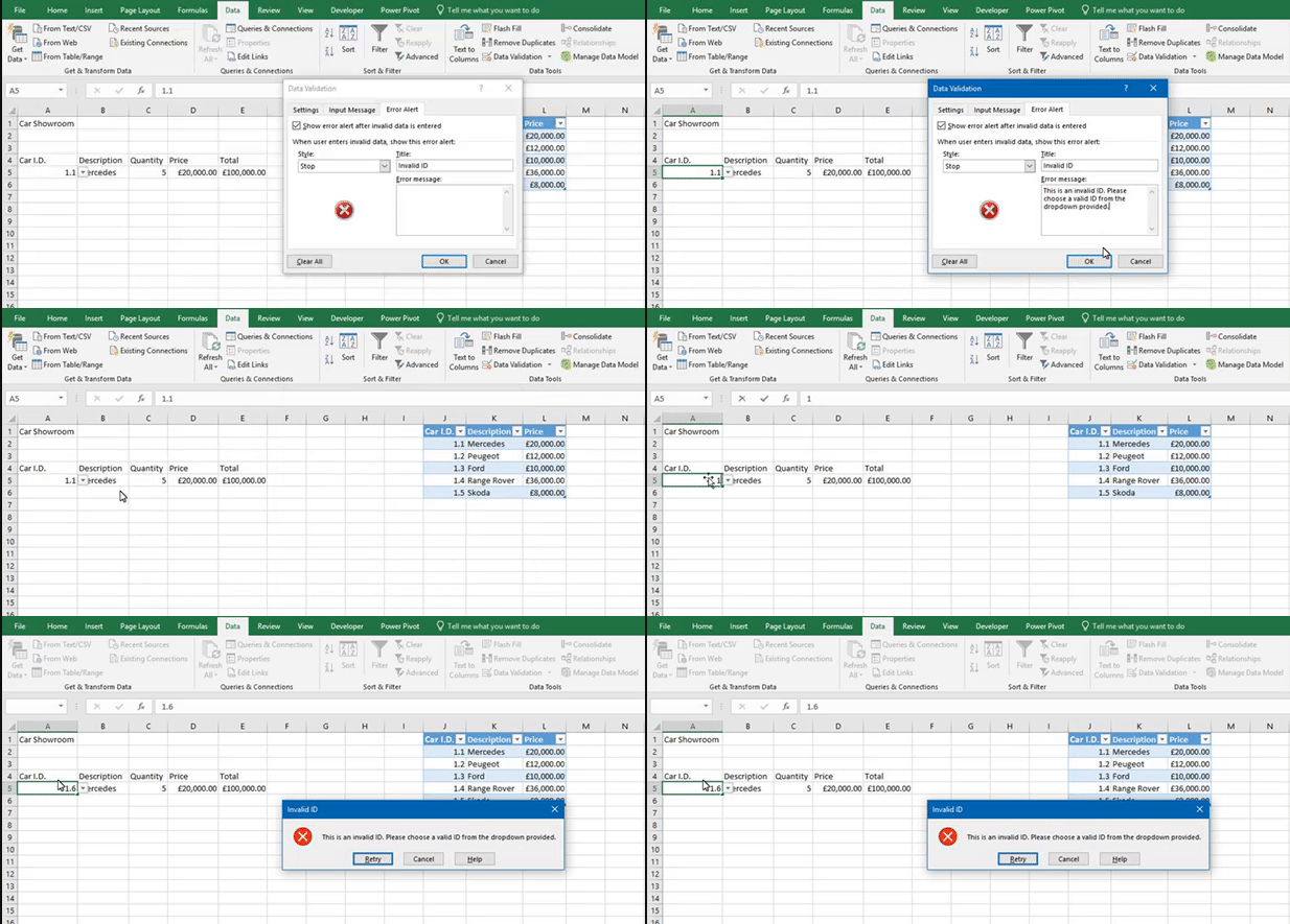
How to create an error alert message


An Error Alert message is a pop up that appears if the user is trying to input data into a cell that isn’t allowed to go into that cell.

To create an Error Alert go to the Data tab and choose Data Validation. Next click on the Error Alert tab. On this tab you will have a dropdown with three options, Stop, Warning and Information.


Stop will not allow wrong data to go into a cell


Warning will warn the user that the data they are trying to input is not allowed to go in that cell but will still give them the option of inputting that data.


Information provides the user more information of what data needs to go in that cell


Once you have chosen one of the above options type a Title and Message into the relevant boxes. Finally click OK.


This content is aimed at the Intermediate level.   Click here to view our course overview.

How to only allow dates in cells using data validation


If you want to restrict users so they can only input dates into cells, then use Data Validation.

Firstly, select the cell(s) that you want to restrict. Then go to the Data tab and select Data Validation. Once selected, go to the Allow dropdown and choose Date. In the Data dropdown select the best option for your spreadsheet. For example, if you want the user to input dates from the past then you need to choose Less Than. Finally, in the Date box type in the criteria. 


This content is aimed at the Intermediate level.   Click here to view our course overview.

How to only allow whole numbers in cells using data validation


If you want to restrict users so they can only input whole numbers into cells, then use Data Validation.

Firstly, select the cell(s) that you want to restrict. Then go to the Data tab and select Data Validation. Once selected, go to the Allow dropdown and choose Whole Number. In the Data dropdown select the best option for your spreadsheet. For example, if you want the user to input whole numbers between two points then you need to choose Between. Finally, in the Values box type in the criteria(s).


This content is aimed at the Intermediate level.   Click here to view our course overview.

How to only allow decimals in cells using data validation


If you want to restrict users so they can only input decimal numbers into cells, then use Data Validation.

Firstly, select the cell(s) that you want to restrict. Then go to the Data tab and select Data Validation. Once selected, go to the Allow dropdown and choose Decimal. In the Data dropdown select the best option for your spreadsheet. For example, if you want the user to input decimal numbers lower than a number that also includes that number, select less than. Finally, in the Values box type in the criteria(s).


This content is aimed at the Intermediate level.   Click here to view our course overview.

How to only allow a specific amount of characters in cells using data validation


If you want to restrict users so they can only input a certain amount of characters into cells, then use Data Validation.

Firstly, select the cell(s) that you want to restrict. Then go to the Data tab and select Data Validation. Once selected, go to the Allow dropdown and choose Text Length. In the Data dropdown select the best option for your spreadsheet. For example, if you want the user to input words that are 8 characters long, choose Equal To. Finally, in the Values box type in the criteria(s), e.g. 8. 


This content is aimed at the Intermediate level.   Click here to view our course overview.

How to apply a drop down using data validation


To create a dropdown in Excel, firstly select the cell that you want to apply the dropdown too. Next go to the Data tab and select Data Validation. This will then open the Data Validation window. On the settings tab select the Allow dropdown and select list. Next, click in the source box and select the range of cells that contain your dropdown content.


This content is aimed at the Intermediate level.   Click here to view our course overview.

How to create an input message


An Input Message informs the user what data needs to go into the selected cell. To create an Input Message, go to the Data tab and select Data Validation. This will then open the Data Validation window. Next go to the Input Message. In the Title box type the title for Message and in the Message box type the message you want the user to read. Finally click OK.


This content is aimed at the Intermediate level.   Click here to view our course overview.

How to stop a column reference changing when dragging a formula across


If you’re referencing a whole column for example B:B and then want to drag the formula across it will change to C:C. If you want the formula to stay refenced to B:B when you drag the formula across then we need to put dollar signs before both letters. For example $B:$B.


This content is aimed at the Introduction level.   Click here to view our course overview.

How to add Subtotals


Subtotals are applied to data using summary functions such as SUM or AVERAGE. To apply subtotals firstly select all your data. Next, go to the Data tab and select Subtotal and this will open the Subtotal window.


At Each Change In – The column that you want to Subtotal

Use Function – The function you want to use to calculate the Subtotal

Add Subtotal To – The column that contains the values you want calculate


Once you have completed the above options click OK. Subtotals will now be applied to your data.


This content is aimed at the Introduction level.   Click here to view our course overview.

How to apply a textbox to your spreadsheet


If you want to add a body of text to your spreadsheet that isn’t typed directly into a cell, then use a text box.

To insert a text box, go to the Insert tab and select Text. From the drop-down choose text box and then draw a text box onto your spreadsheet. 

To add text to your text box, click in it and start typing.  


This content is aimed at the Introduction level.   Click here to view our course overview.

Naming a single range using the Create from Selection tool


If you want to create a named range from a selection of cells, then a quick way of doing this is using the Create from Selection tool. Select the cells you want to name and then go to the formula tab and select Create from Selection. The Create Names from Selection options box will then appear. Choose the option of where the name for your range is located. For example, if the name for your range is in the first column, choose Left Column. 


This content is aimed at the Advanced level.   Click here to view our course overview.

Naming multiple range using the Create from Selection tool


If you want to create multiple named ranges from a selection of cells, then a quick way of doing this is using the Create from Selection tool. Select the multiple rows and columns you want to name and then go to the formula tab and select Create from Selection. The Create Names from Selection options box will then appear. Choose the option of where the name for your range is located. For example, if you want to create named ranges based on the headers at the top and the first column then select Top row and Left column. 


This content is aimed at the Advanced level.   Click here to view our course overview.

How to copy just the Subtotals


If you only want to copy subtotals from your data, then you can’t do a straight forward copy and paste as it will paste all the hidden data as well. Instead, select all the subtotals and press F5. This will then open the Go To window and in this window select Special. Next, in the Go to Special window select Visible Cells Only, then click OK. The final step is to copy the subtotals and paste it. This will now only copy and paste the subtotals and not all the data.


This content is aimed at the Introduction level.   Click here to view our course overview.

How do I find a specific word or phrase in Excel?


If you’re looking for a certain word or phrase in a spreadsheet, then how about using the Find tool. It’s a handy tool where you type the word you want to find and then Excel will find the word in your spreadsheet.

You will find the Find tool on the Home tab, in the Editing group.


This content is aimed at the Introduction level.   Click here to view our course overview.

How to Find and Replace text in Excel?


If you want to replace the values of cells with something else, why not give the Replace tool a go.

Just type in the word that you want Excel to replace and then type in the word you want to replace the text with.


This content is aimed at the Introduction level.   Click here to view our course overview.

How to identify invalid data in Excel?

If you want to find data that has been incorrectly inputted, then use the simple to use Circle Invalid Data Tool. This circles any incorrect data.


How to use the Circle Invalid Data tool

1. Go to the Data tab, Data Tools and select the Data Validation dropdown.

2. Select Circle Invalid Data.


This content is aimed at the Intermediate level.   Click here to view our course overview.

How to input a value in Excel that starts with a zero?


As you might have noticed, you can’t start a number in excel with a zero. There is way simple way of getting around this. Just place an apostrophe (‘) before your number. This will keep the zeros at the beginning of your number.


This content is aimed at the Intermediate level.   Click here to view our course overview.