If you want to filter using a broader criterion then you can use question marks in your search. A question mark represents a character and you use them within the search bar on your filter dropdown.

For example, if you typed 10?4 into the search bar it would return numbers such as 1004, 1014, 1024, 1034 etc.

If you want to filter data more broadly, then why not use an Asterisk Wildcard to help. An asterisk represents multiple characters when filtering. In the search bar on your filter dropdown you can place the asterisk in different places to return different outcomes. For example:

*A would return all records that end in A

A* would return all records that start with A

H*A  would return all records that start with H and end in A

*A* would return all records that has a A in it

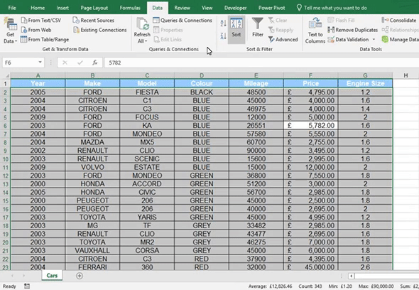
In Excel you can sort multiple columns of data. This allows you to sort your data more thoroughly. 

To sort multiple columns, firstly select all your data. Next, go to the data tab and select sort, this will then open the Sort Window. In the drop down next to Sort by, select the column that you want to sort first. In the Sort On drop down select values. For the Order drop down choose how you want the data to be sorted.

Once you have completed that level of drop downs click on add level. Repeat the process above and keep doing it until you have sorted all the columns you want to sort.

Before clicking OK, make sure that the My Data has Headers box is ticked. Otherwise it will sort your headers in with the rest of your data.

Your data should now be sorted by the specified columns.

If you want to be able to filter your data, then we firstly we have to apply filters to your data. 

To apply filters, select your data and go to the Data tab. On the ribbon you will find the Filter button. Click on it and you will notice dropdowns will get applied to your headers. 

If you want to filter data, then you can use the check boxes in the AutoFilter drop downs to do so.

To filter this way, click on a filter drop down and then deselect select all. This will deselect everything. Next check the options you want Excel to return and then click OK.

One way of filtering data is using the search bar located in the AutoFilter drop down. To use it go into the dropdown and click in the search bar. Next, type in the item that you are searching for and then click OK.

Once you have finished filtering a column of data, you can then clear the filter. To do this, select the dropdown that the filter has been applied to and then select Clear filter from “ “. This will then clear the filter from that column. 

Once you have finished filtering multiple columns of data, you can then clear the filters. To do this, go to the data tab and on the ribbon select Clear. This will then return you with all your data.

You can use slicers to filter data that is formatted in a table quickly and easily. To insert a slicer into your Excel spreadsheet, select your table and go to the Insert tab. In the Filters group select Insert Slicer and choose the fields from the list you want a slicer to apply too.

You will now have a slicer in your spreadsheet. To use it, just select the option from the list that you want to view. For example, above I have chosen to see the food orders that Terry Walton dealt with.

If you are finding it difficult to find information from a data source, you can sort it into alphabetical order.

How to Sort Your Data

1. Select the data you want to sort

2. Go to the Data tab > Sort and Filter Group and select the Sort A-Z icon for your data to be in alphabetical order, or the Z-A icon if you want it in reverse alphabetical order.