Instead of using a cell range as your table array, you can use a table name. The benefits of doing this is that if you add more data to your table it will automatically pull it across into your formulas.

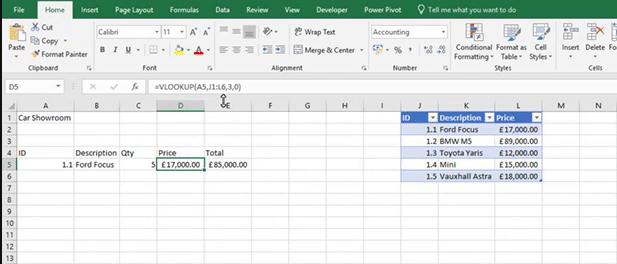
In a standard VLOOKUP your formula would be something like the one below.

 =VLOOKUP(A5,Sheet7!A2:D50,2,0)

If you want to use a table name, i.e Cars, in your VLOOKUP formula then it would look something like the one below.

=VLOOKUP(A5,Cars,2,0)

If you want to make your data easier to work with then why not place it into a table format. To do this select the data and go to the Insert tab. Next, select Table on the Ribbon and this will open the Create Table window. In this window it will have the range of cells you want to convert to a table and a box that says My Table has Headers. If your table has headers, make sure that box is ticked. Then click ok.

You can give a cell or range of cells a unique name which can then be used in formulas or to find cells.

To create a named range, select the cell(s) that you want to apply a name to. Then click in the Name Box and type in the name you want to give the cell(s). Once you have done that press enter. 

Named ranges must have a unique name.

If you want to edit a named range, go to the Formulas tab and select the Name Manager in the Defined Names group. 

In Name Manager select the named range you want to edit and select Edit. You can then change the name of the range, any comments about the named range and the range of cells that the name range covers.