How to work out an average based on two criteria’s?


If you want to be able work out the average based on multiple criteria, then we can use the AVERAGEIFS formula. 


The Syntax for this formula is:


Average Range – the range of numerical values you want to calculate the average from


Criteria Range 1, Criteria Range 2... – the data ranges that you will find the criteria’s


Criteria 1, Criteria 2... - the items that you want to find in the criteria ranges to be able to calculate the average.


This content is aimed at the Advanced level.   Click here to view our course overview.

How to hide a Row/Column


If you want to hide a particular row or column in excel, you right click on the row/column you want to hide, press hide on the drop down menu.

To un-hide the column, you double left click between the two numbers or letters and it will re-appear.


This content is aimed at the Introduction level.   Click here to view our course overview.

How to add a theme to your spreadsheet


If you want to change the look of your Excel workbook, then have a look at applying a theme. A theme allows you to change the colours, fonts and effects in your workbook. 

To apply a theme, go to the Page Layout tab and select Themes. From the dropdown choose a theme that you would like your workbook to have.


This content is aimed at the Introduction level.   Click here to view our course overview.

How to change your themes colours in Excel


If you want to change a theme’s colours you can choose a different colour scheme. 

To choose a different colour scheme go to the Page Layout tab and select Colors. From the dropdown choose a colour scheme that you like.


This content is aimed at the Introduction level.   Click here to view our course overview.

How to change your themes fonts in Excel


If you are not happy with the fonts that your theme uses, then you can change them.

To do this go to the Page Layout tab and select Fonts. From the dropdown choose a font option that you like.


This content is aimed at the Introduction level.   Click here to view our course overview.

How to change your themes effects in Excel


If you are not happy with the effects that your theme uses, then you can change them.

To do this go to the Page Layout tab and select Effects. From the dropdown choose an effect option that you like.


This content is aimed at the Introduction level.   Click here to view our course overview.

How to create your own colour scheme in Excel


If you don’t like the colour schemes that Excel provides then you can create your own colour scheme. 

To create your own colour scheme, go to the Page Layout tab and select Colors. At the bottom of the dropdown select Customise Colors. This will then open the Create New Theme Colors window. Finally go and choose different colour for your Accents and Hyperlinks.

To finish give your new colour scheme a name by typing it into the Name box and then click Save.


This content is aimed at the Intermediate level.   Click here to view our course overview.

How to create your own fonts in Excel


If you would like to create your own font combinations instead of using Microsoft’s options, then go to the Page Layout tab and select Fonts. In the dropdown select Customize Fonts. This will open the Create New Theme Fonts window.

In the Heading Font dropdown, select a font you want to use for your headings.

In the Body Font dropdown, select a font you want to use for the body of your text.

In the Name box, give your font combination a name and click Save.


This content is aimed at the Intermediate level.   Click here to view our course overview.

What happens if I have hashes (####) in a cell


If you see several hashes in a cell, then don’t panic. All it means is the data in that cell is too big for the cell. So, to remove the hashes, widen the column the hashes are located in. 


This content is aimed at the Introduction level.   Click here to view our course overview.

How to Autofit an entire spreadsheet?


If you don’t want to go and autofit all your columns individually, then how about adjusting all your columns in a sheet at once. Firstly, click on the Select All icon in the corner. Once your spreadsheet is selected, double click in between one of the letters on your headers.


This content is aimed at the Introduction level.   Click here to view our course overview.

How to Autofit multiple columns?


If you want to adjust multiple column widths, then why not use the Autofit tool to help. Just select the columns you want to resize and double click in between two of the letters within the selected columns. 


This content is aimed at the Introduction level.   Click here to view our course overview.

How to Autofit a column width?


If your column isn’t wide enough for the values then why not use the Autofit tool. Just double click in the middle of two letters on your headers. This will then adjust your column width.


This content is aimed at the Introduction level.   Click here to view our course overview.

How do I add together hours in Excel?

Excel allows you to add up hours, we just use a Sum formula. But when we have added enough hours to give us an answer over 24 hours, it doesn’t show the true number of hours we’ve got. For example, if we’ve got an answer of 28 hours, it will show in Excel as 04:00. This means 1 day 4 hours. To get Excel to show it as 28:00, we need to change the formatting.


So we go to Number Formats, custom and we place square brackets i.e.[ ] around the hh of the format.


This content is aimed at the Introduction level.   Click here to view our course overview.

How to apply a colour to a cell that automatically changes colour?

Excel lets you apply a colour to a cell that will change if it meets certain criteria, this is called Conditional Formatting. You will find the Conditional Formatting tool on the Home tab. If you select it and choose Highlight Cell Rules, you can choose the rule that you want to apply.


For example, if you want a cell that contains a number that is greater than 10 to go green, then select the Greater Than option, then type in the value 10 and select the colour green from the dropdown.


This content is aimed at the Introduction level.   Click here to view our course overview.

How do I show duplicate values in a range of cells using colours?


If you want to show duplicates clearly, how about using the Conditional Formatting tool to show the duplicates with colour.

All you need to do is select Duplicate Values from the Conditional Formatting tool and choose a colour. The duplicates will now be showing in colour.


This content is aimed at the Introduction level.   Click here to view our course overview.

How do I show unique values in a range of cells using colours?


If you don’t want to spend time going through data to find unique values, how about using the Conditional Formatting tool to show the unique values with colour. It’s rather simple to apply, select the Conditional Formatting tool and select duplicate values from the Highlight Cell Rules menu.

Once there, change Duplicate to Unique and select a colour. Your unique values should now be colour.


This content is aimed at the Introduction level.   Click here to view our course overview.

How do I show values that are above average in colour?


If you want to show values that are above average more clearly, then why not try the Above Average tool located in Conditional Formatting.

It quickly applies a specified colour to the cells which are above average that are selected at the time.


This content is aimed at the Introduction level.   Click here to view our course overview.

How do I show values that are below average in colour?


If you want to show values that are below average more clearly, then why not try the Below Average tool located in Conditional Formatting.

It quickly applies a specified colour to the cells that are selected at the time.


This content is aimed at the Introduction level.   Click here to view our course overview.

How do I remove / apply lines on my spreadsheet?


By default, Excel always opens with gridlines. If you don’t want to see gridlines then how about removing them.

To remove gridlines, just untick the Gridline check box on the View tab. It will then remove the gridlines.


This content is aimed at the Introduction level.   Click here to view our course overview.

How to remove / apply the formula bar in Excel?


If you don’t use the formula bar, then how about removing it from your screen. Go to the View tab and un-tick the Formula Bar check box.

This will remove the formula bar. If you want the formula bar to appear again, tick the formula bar check box.


This content is aimed at the Introduction level.   Click here to view our course overview.

How to remove / apply the headings in Excel?


If you open Excel and your headings are not there to help you determine which cell you’re in, then we can quickly apply them.

Select the View tab and check the Headings check box. Your headings should now be applied.


This content is aimed at the Introduction level.   Click here to view our course overview.

What do I do if my headings are numbers instead of letters in Excel?


If your column headers in Excel are showing as numbers, don’t worry. You can fix this in a few steps.

Select the File tab, Options, Formulas and untick the R1C1 reference style box. Your column headers will now show as letters.


This content is aimed at the Introduction level.   Click here to view our course overview.

How to remove duplicates?


If you want a list of unique data entries, then you can use the Remove Duplicates tool to remove any duplicates in that list. Just select the data you want to remove duplicates from, then select Remove Duplicates located on the Data tab.

If you have multiple columns selected at a time then you can choose which column you want to remove duplicates from.


This content is aimed at the Introduction level.   Click here to view our course overview.

How to edit multiple sheets at once


Editing data on multiple spreadsheets can be time consuming. So how about editing multiple spreadsheets at once. To do this, select the sheets that you want to edit and start editing.

For example, if I want the data in cell A4 on sheet one to be the same as cell A4 on Sheet 2, I would select sheet 1 and 2 and type into A4 the data I want.


This content is aimed at the Introduction level.   Click here to view our course overview.

How to find cells that contain data validation in Excel?


When applying dropdowns through data validation in Excel, when you click out of the cell the dropdown arrow disappears, therefore you don’t know which cells contain data validation. To make it easier to find data validation such as dropdowns in excel we can use the Find and Select tool on the Home tab.

We can then select Data Validation from the list. All cells that contain data validation will now be selected.


This content is aimed at the Introduction level.   Click here to view our course overview.

How to find cells that contain formulas in Excel?


If you want Excel to show you cells that contain formulas why not use the Find and Select tool located on the Home tab.

Then select formulas, and all formulas in that spreadsheet will be selected.


This content is aimed at the Introduction level.   Click here to view our course overview.

How to find cells that contain Comments in Excel?


If you want Excel to show you cells that contain comments, why not use the Find and Select tool located on the Home tab.

Then select Comments, and all comments in that spreadsheet will be selected.


This content is aimed at the Introduction level.   Click here to view our course overview.

How to find cells that contain conditional formatting in Excel?


If you want Excel to show you cells that contain Conditional Formatting, why not use the Find and Select tool located on the Home tab.

Then select Conditional Formatting, and all Conditional Formatting in that spreadsheet will be selected.


This content is aimed at the Introduction level.   Click here to view our course overview.

How to find cells that don’t contain formulas in Excel?


In Excel, a cell that does not contain a formula is known as a constant. If you want to find where these constant cells are located, then we can use the Find and Select tool located on the Home tab.

Once there, select Constant and it will show you all the cells that do not contain a formula.


This content is aimed at the Introduction level.   Click here to view our course overview.

How to find the nth smallest number in a range?


If you want to find the smallest number in a range, you could use the MIN formula. Unfortunately, it limits you to only being able to find the smallest value. However, you could use the SMALL formula. This will find the smallest number that you specify. For example, if you want to find the 3rd smallest number in a range, you can.


This content is aimed at the Introduction level.   Click here to view our course overview.

How to find the nth largest number in a range?


If you want to find the largest number in a range, you could use the MAX formula. Unfortunately, it limits you to only being able to find the largest value. However, you could use the LARGE formula. This will find the largest number that you specify. For example, if you want to find the 3rd largest number in a range, you can.


This content is aimed at the Introduction level.   Click here to view our course overview.

How do I compare two strings of text to see if they are the same?


If you want to compare two strings of text, then try the EXACT function in Excel. The EXACT function compares a string of text with another one. If they are the same then Excel will return an answer of TRUE.

If they are not the same then Excel will return FALSE. Be aware that the EXACT function is case sensitive.


This content is aimed at the Introduction level.   Click here to view our course overview.

How do I find text within text?


In Excel, we can use the Find formula. The formula looks through a string of text to find what you have asked for it to find. Excel will then return a number which symbolises the position of the text within a string text. In the image above we have Excel to find ‘b’. Excel has then returned 11 as b is the 11th character across. Be aware that the FIND function is case sensitive.

In the image above we have asked Excel to find the word ‘the’. Because it hasn’t got a capitalised ‘t’, Excel has returned 33 which shows the position of the second ‘the’ in the sentence.


This content is aimed at the Introduction level.   Click here to view our course overview.

How to align text in Excel?


If you want to tidy up or reposition your text in a cell, then why not check out the alignment tools. These tools will allow you to position your text in various places in cell. Just select the cells you want to realign and then select the correct alignment tool for you.


This content is aimed at the Introduction level.   Click here to view our course overview.

How to apply diagonal borders?

If you need a row and column header in the same cell, then how about using a diagonal border to achieve this. Just select More Borders in your borders dropdown and select the diagonal line you want to apply.


This content is aimed at the Introduction level.   Click here to view our course overview.

How to hide individual cells?


Do you want to hide cells without having to hide the entire row or column? Then why not try this handy trick. Select the cells you want to hide and go to Format Cells. Choose Custom and then type three semicolons (;;;). This will hide your data.


This content is aimed at the Intermediate level.   Click here to view our course overview.

How to erase borders in Excel?


Have you got unwanted borders in your spreadsheet? How about trying the Erase Border tool? It’s easy to access and use. Just go to the Borders icon on your ribbon and select Erase Border from the dropdown. Then use the eraser icon to remove the borders you don't want.


This content is aimed at the Introduction level.   Click here to view our course overview.

How to change the colour of cell borders?


So, you want to change the colour of your borders. Just select the Borders tool and click Line Coluor, then select a colour from the options provided. If you’re not happy with the colours provided, click on more colours to get a wider range of colours.    


This content is aimed at the Introduction level.   Click here to view our course overview.

How to change how a border looks?


If you don’t want a straight-line border, then how about having a look at some of the other options Excel provides. Just select the Borders tool and go down to Line Styles and choose a style that you like.


This content is aimed at the Introduction level.   Click here to view our course overview.

How to change the direction of my text in Excel?

If you want to make text, such as headers, take up less room in your spreadsheet, then use the orientation tool. This will allow you to view more columns at a time.
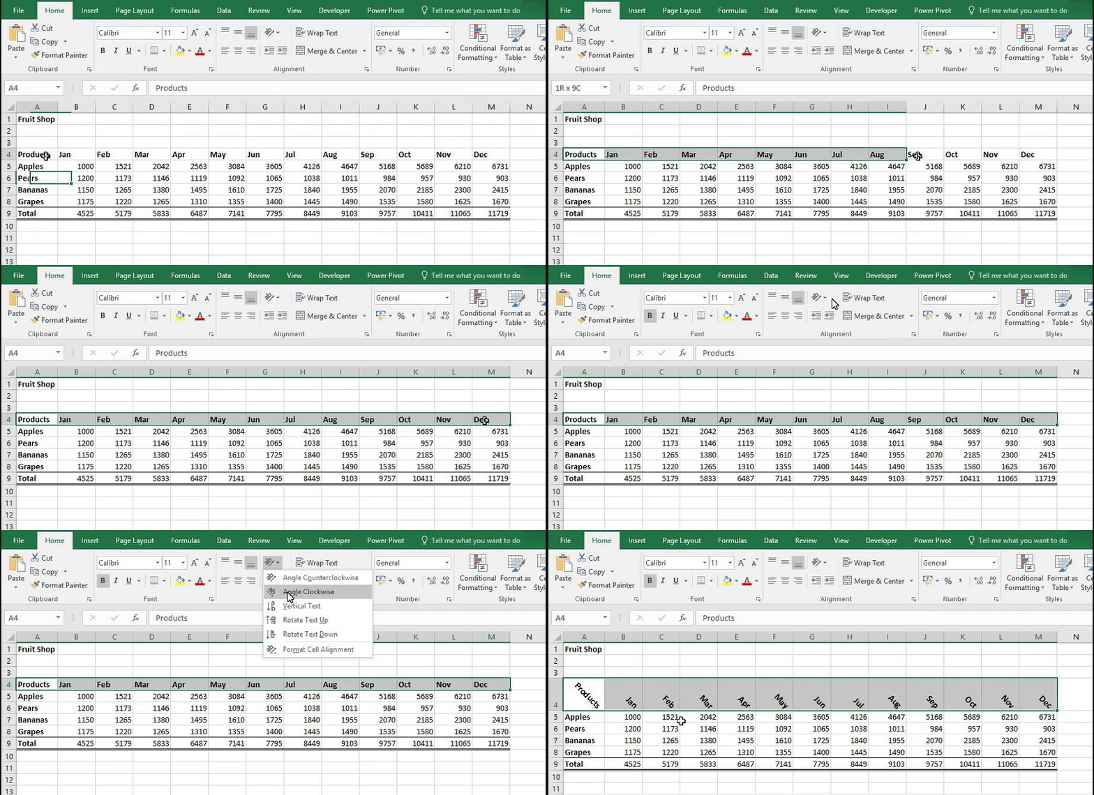

How to Change the Orientation

1. Select the cell(s) that contain(s) the text you want to change the direction for.

2. Go to the Home tab, Alignment and select the Orientation tool.

3. Choose the orientation you want to apply.


This content is aimed at the Introduction level.   Click here to view our course overview.

How do I clear formats from a cell in Excel?

Try the Clear Formats tool, it clears the format of your cell without deleting the value of the cell.


How to clear formats

1. Select the cell(s) that you want to clear the formatting from.

2. Go to Home tab, Editing and select Clear.

3. Choose Clear Formats from the dropdown.


This content is aimed at the Introduction level.   Click here to view our course overview.

How do I apply pound signs to values in Excel?

Instead of having to type out the pound sign repeatedly, Excel has provided a formatting tool that will take care of it for you.


 How to apply pound signs

1. Select the values you want to apply pound signs too

2. Go to the Home tab, Number and select the drop down box

3. Select either Currency or Accounting to apply pound signs


This content is aimed at the Introduction level.   Click here to view our course overview.

How to decrease the number of decimal places of a value in Excel?

If you have too many decimal places showing, you can quickly adjust a value so it shows less decimal places by using the Decrease Decimal tool.


How to use the Decrease Decimal tool

1. Select the values that you want to decrease the decimal places of.

2. Go to the Home tab, Number and click on the Decrease Decimal tool until you have the number of decimal places you want.


This content is aimed at the Introduction level.   Click here to view our course overview.

How to increase the number of decimal places of a value in Excel?

If you have too few decimal places showing, you can quickly adjust a value so it shows more decimal places by using the Increase Decimal tool.

How to use the Increase Decimal tool

1. Select the values that you want to increase the decimal places of.

2. Go to the Home tab, Number and click on the Increase Decimal tool until you have the number of decimal places you want.


This content is aimed at the Introduction level.   Click here to view our course overview.

How do I change the font in my spreadsheet?


Are you happy with the way your text looks in Excel? If not, then you can choose a different font from the many that Excel provide. Just select the text you want change the font of, then go to the Home tab > Font and select a font from the Font dropdown. 


This content is aimed at the Introduction level.   Click here to view our course overview.

How do I change the size of my text?

If you want to change the size of your text, its straight forward. Select the text you want change the size of, then go to the Home tab > and choose a number from the Font Size drop down. The bigger the number you choose, the larger the text will be. 


If you don’t want to use the drop down to increase and decrease your font size, you can also use the Increase Font Size and Decrease Font Size icons. 


This content is aimed at the Introduction level.   Click here to view our course overview.

How do I change the colour of a cell in Excel?

Do you want to add colour to your spreadsheet? Then use the Fill Colour tool located on the Home tab in the Font group. To use the Fill Colour tool, select the cells you want to apply colour too, then click the Fill Colour tool and choose a colour from the drop down provided.

If you’re not happy with the range of colours provided, how about selecting More Colours to get a larger variety of colours.


This content is aimed at the Introduction level.   Click here to view our course overview.

How do I change the colour of text in Excel?

Do you want to add colour to your text in a spreadsheet? Then use the Font Colour tool located on the Home tab in the Font group. To use the Font Colour tool, select the cells you want to apply colour too, then click the Font Colour tool and choose a colour from the drop down provided.

If you’re not happy with the range of colours provided, how about selecting More Colours to get a larger variety of colours.


This content is aimed at the Introduction level.   Click here to view our course overview.

How to show all text in a cell without changing the cell width?

If you want to show all the text in a cell without having to alter the cell width, then use the Wrap Text tool. It’s easy to use, just select your text and click on the Wrap Text tool located on the Home tab in the Alignment tool.


This content is aimed at the Introduction level.   Click here to view our course overview.

How to merge cells together in Excel?

Merging cells together is straight forward. Select the cells you want to merge and click on the Merge and Center tool located on the Home tab in the Alignment group. Your cells will now have merged. 

If you want to unmerge your cells, select the merged cell and click on the Merge and Center tool and choose Unmerge Cells. 


This content is aimed at the Intermediate level.   Click here to view our course overview.

How do you apply borders to a cell in Excel?

Excel has a tool called Borders which applies lines to your spreadsheet.

How to use borders:

1. Select the cell(s) you want to apply a border too.

2. Go to the Home tab, Font and select the Border tool dropdown.

3. Choose the border you want to apply.


This content is aimed at the Introduction level.   Click here to view our course overview.

How do you copy formatting from one cell to another?

Try the format painter, it’s simple to use and copies the format of the cell rather than the contents. When you are adding new columns or rows, it’s the quickest way to ensure you match the formatting.


How to use Format Painter:

1. Select the cell you want to copy formatting from.

2. Go to the Home tab, Clipboard and select the Format Painter tool.

3. Select the cell(s) you want to apply the formatting too. 


This content is aimed at the Introduction level.   Click here to view our course overview.